
DLP Slicing::11.23.2016+15:08
A couple months ago I was talking to a former coworker, Chad Hamlet, about 3D printing and he brought up a gripe he had with his workflow where it would take hours (potentially 12+ hours) to generate the slices he needed to use as input for his DLP printer. To put things into perspective, the actual prints take as long, if not much longer depending on what’s being printed. My kneejerk reaction was that this was ridiculous and that he should be able to generate slices in a significantly shorter time, especially with GPU acceleration. He mentioned that there was a prototype app that was done during a hackathon at Formlabs, but he couldn’t get it working for large models with millions of polygons (his ZBrush output). With the knowledge of how that slicer worked, I started on making a standalone one in C++ that could handle his workloads.
Slice Generation
For the slice generation algorithm to work, the model has to be water-tight (manifold). This means that there aren’t any discontinuities in it, the reason for which should become clear soon. This presents some problems when printing because it normally means that the user has to do a bunch of CSG operations to carve out holes for the resin to drip out of. As it turns out, there’s actually some tricks that you can use to make holes without doing CSG. Additionally, the model can have multiple overlapping and intersecting pieces as long as each piece is water-tight.
The general idea of the algorithm is to continuously slice through the model taking note of what’s “inside” and “outside”. To do this analytically, it would be insanely expensive and take a really long time and you’d probably use something like raytracing. Instead we use the GPU and the stencil buffer to accelerate this, since most GPUs can render millions of triangles in a couple milliseconds.
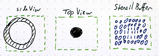
To start out, let’s envision the intial setup of the world. There’s a model, in this case a hollow sphere, positioned in the center of our camera volume, which we’ll take to represent the print volume. We’re seeing this from the side, and the left is the bottom (far plane of the camera) and the right the top (near plane). To generate the slices, we’re going to render this model while sliding the camera volume toward the top end (but not change the size or shape of the volume). Our rendered slice will look like the intersection of the bottom of this volume and the model.
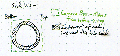
In this implementation, we’ll be using the stencil buffer, which is a pretty old hardware feature that allows us to do math by rendering geometry. If you’ve played Doom 3 or any idTech 4 games, you’ve seen this in action as they use the stencil buffer to render out their shadows. In fact, they are also concerned with knowing the inside of models versus the outside. For this algorithm, we’re going to start by disabling face culling; normally you’d only want to render front faces but we need both front and back faces. Then, we configure the stencil buffer operations such that whenever a front face is rendered, we decrement the value in the buffer while wrapping around (the stencil buffer holds unsigned integers), and when a back face is rendered, we increment and wrap. What this means is that any geometry that doesn’t have a matching “other side” will leave a non-zero value in the stencil buffer. Since we’re slicing through the model, the intersection of the model and the far plane will do exactly that. To get the actual rendered slice, we then just need to draw a white plane masked against the non-zero stencil buffer.
Optimization, Improvements, Tricks
The Formlabs implementation does quite a bit of unnecessary work, namely rendering the model three times: once with front-faces, once with back-faces, and then a third time to actually render the slice. In my implementation I only render it once because it’s possible to configure the hardware to handle front and back faces in one pass. The third pass is also complete overkill since you just need to mask something against the stencil buffer. A single, fullscreen triangle is enough here; there’s no need to re-render the model. For a tiny model this optimization won’t really make a difference, but for something with millions of triangles, it’s the difference between 5 minutes and 15.
Something my coworker pointed out was that adding antialiasing to the slices would result in various levels of partially cured resin on the edges of the object, meaning that you can get a significantly smoother surface versus just black and white. To this end, I added support for using MSAA for antialiasing. The program will detect and clamp this setting accordingly, but there are some broken drivers out there that report being capable of MSAA but then crash when actually using it.
The final slices get saved out to disk as PNGs. Something worth noting is that PNG has a subformat for 8-bit per channel greyscale images. Since we’re going to be rendering greyscale images, it’s important to use this instead of the standard RGBA, 32-bit format. This will both cut down the amount of disk space required and the amount of time it takes to compress the slices.
Some miscellaneous features include being able to specify all of the parameters of the printer in the config file, being able to scale the model (useful for testing or if you’re not modelling in the same units as the output), and validation of the model against the print volume.
I mentioned earlier that it’s possible to avoid doing CSG operations on the mesh but still punch holes in it, which is useful when you want to duplicate, scale, and invert the model to make a shell. To do so, you duplicate the polygons on both surfaces where you want the hole to be and invert the normals of each side. This will, in effect, make it so that that part of the surface always has both a front and back face, leaving an opening. These don’t have to be manifold as long as their edges are aligned on the up axis (Z in the case of this program).
Results
On my GTX 1080, I’ve timed a five million triangle model as taking around three minutes to slice (~4000 slices). This is over 240 times faster than the software that my coworker was previously using. So I consider all of this to be pretty successful. I was originally going to make the program multithreaded so the CPU could build up a frame or two of data while waiting for the GPU to render, and also make the image compression and saving happen in a different thread. These could be added and it would generate the slices even faster than it does now. Switching to a modern API like Vulkan (it uses OpenGL right now) would enable further speed increases since transferring the rendered image back to the CPU could be done in an asynchronous way (it’s synchronous in GL). I’ll leave these as exercises for the reader.
Chad sent me a bunch of pics (you can see more on his blog) and I’ve reproduced a few of them here to show off the nice result that he was able to get.
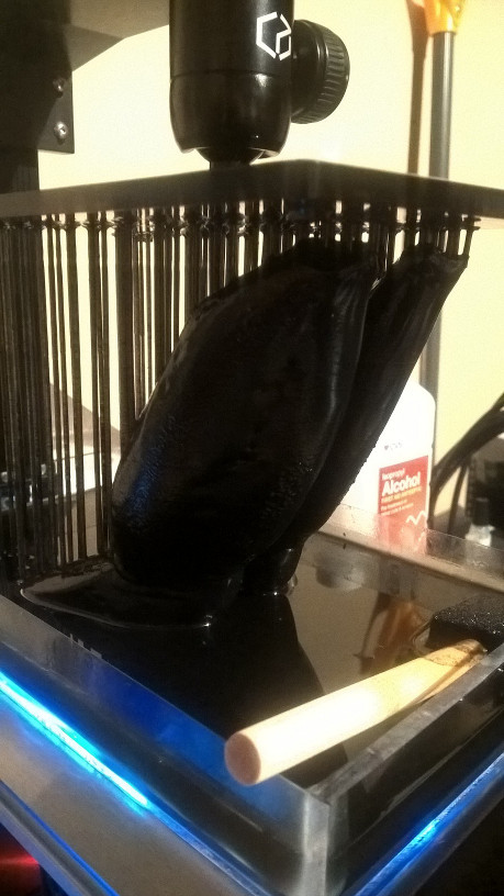 |
 |
 |
Get It
I’ll be making a packaged version available soon, but I need to draft up an appropriate freeware license. If you’re a programmer, though, you could pretty easily write your own version from this description. Feel free to contact me with any questions about how it works.
dib - future::10.06.2016+14:12
In the previous post, and the one before that I talked about the architecture and motivations for writing my build system, dib. In this post I’m going to go over some sticking points, bugs, and missing functionality that I’m planning on remedying in the future.
General Items
- Stop on Failure/Partial Success - Currently, dib won’t stop on failure immediately and won’t record partial successes in the database. This is pretty awful, especially for larger codebases since it will do full rebuilds of the affected Target until it builds correctly. This should be relatively easy to fix, but it’s going to be a bit of a nuanced solution.
- Reduce Database Size - The various databases are larger than they need to be right now. I’m using Data.Text as keys in a lot of places and should be using hashes instead since 32 and even 64 bits is significantly smaller than the smallest file paths will be.
- Target Validation - There are some obvious aspects of Targets that should be validated: ensuring that there’s at least one Stage and one Gatherer. Fixing this at the type level is the obvious best answer, and it looks like there’s already a library for non-empty lists. There might be other things that can be put through validation too, but I need to investigate more here.
- Dependency Caching - There’s no caching at the dep scanner level right now and it leads to a lot of repeated work, especially if one of the dependencies has a significant number of its own dependencies. I don’t have a solid architecture for how I want to handle this yet; I’m leaning toward changing the type signature of the DepScanner function to include the database, but I think it needs something stronger, probably involving the StateT monad.
- Windows Fixes - I have a local fix for this that I need to push, but currently the dib driver program doesn’t make the correct commandline to be executed by “system”, so it fails to run the actual build. There might be other issues with Windows that I don’t know about; I don’t ever test dib there.
C Builder Items
- Better C/C++ Flags Separation - There’s no separation between the flags that are used for C files and the flags used for C++ files. This should be an easy fix with minimal overhead.
- Link Flag Changes Shouldn’t Cause Full Rebuilds - Right now, if the user changes any of the options to the C Builder, it will cause a full Target rebuild. This is obviously not a good thing. I think the solution for this will be adding per-stage hashes which influence the compilation similar to how the Target hash currently does.
Possible Extensions
These are not guaranteed features, but are instead things that could end up in dib, depending largely on how much time and effort I’m willing to put in for them.
- Retrieving Output of a Target’s Last Stage in a Subsequent Target - At the moment, Targets can’t send any information from one to another. I could see this being used to inform a further Target where a library was built to, or something of that sort. However, I’m not really convinced this is a worthwhile feature, since the user can already predict where the output will end up and modify the Targets accordingly. It’s just a possibility I’ve been throwing around.
- Output Caching - Some transforms can be expensive to build: compression of textures, videos, archiving operations, etc… In a multiple user situation it would be advantageous to cache these files somewhere so other users don’t have to endure the lengthy build process if the data hasn’t changed. Being able to have a shared network location (folder, webDAV, ftp) where this cache lives and being able to pull from it would be a really useful feature. This would currently be a lot of work and would require hashing the actual file contents instead of just checking timestamps. I’d want to implement it as an optional feature that could be enabled per-Target.
dib - architecture::09.29.2016+14:47
Last time, I talked about my motivations for writing dib, my personal build system. This time we’re going to examine in depth the underlying architecture, with a focus on the types and execution.
Types
There are four fundamental types that form the structure of a build in dib (in order of increasing abstractness): SrcTransform, Gatherer, Stage, and Target. The first of these, SrcTransform represents the input and output of a command. There are four type constructors which represent the possible relationships of input to output:
- OneToOne - e.g. copying a file from one place to another, or building a .cpp into a .o file.
- OneToMany - e.g. extracting an archive, or writing out a converted file and some metadata
- ManyToOne - e.g. linking .o files into an executable, or archiving a bunch of files.
- ManyToMany - I don’t have any accessible examples for this, but I’ve seen use cases in my professional work.
Pipeline Overview
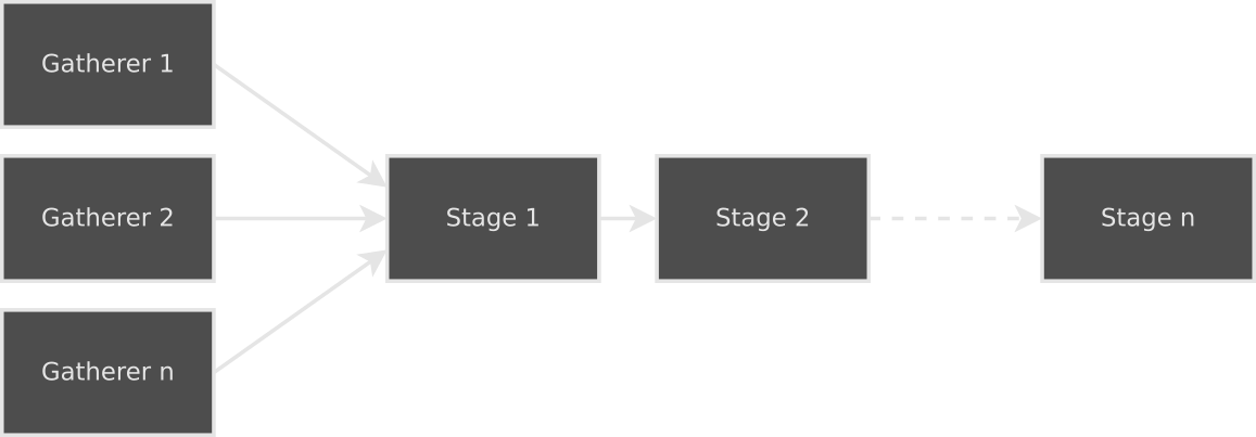
SrcTransforms are the actual data that the build is processing. They are the input to the entire process and are transformed as they move through each segment of the pipeline. They are initially generated by Gatherers. The Gatherers provided with dib only produce OneToOne transforms, the input being the files they gathered, with an empty string as the output. A Target can have more than one Gatherer; the output of each will be combined into a single list that is passed into the first Stage. Each of these Stages then does processing on the transforms that are passed in and passes them to the next Stage.
Stages
Each Stage takes as input a list of SrcTransforms and outputs either a list of SrcTransforms or an error string. At the beginning of every Stage sits an InputTransformer: a function that transforms the list of SrcTransforms into another list suitable for that Stage to process. In contrast to the other parts of a Stage (as we’ll soon see), this operates on the entire list to easily enable collation. The built-in C/C++ builder, for example, collates the list of OneToOne transforms of object files into a ManyToOne of object files to executable/library.
After passing through the InputTransformer, each SrcTransform is individually passsed into a DepScanner, an IO action that takes a SrcTransform and produces a SrcTransform. In the case of the C/C++ builder this is the CDepScanner, which recursively scrapes the includes for further, unique includes. It changes the input OneToOne transforms into ManyToOne and adds the dependencies after the actual source file to be built. When processing a Stage, the timestamps of the input files of each transform are checked to determine if the transform should be built. By adding the dependencies to the transform, the system takes care of rebuilding that transform when they change, for free.
The final piece of the Stage is the StageFunc, which is the actual business logic that executes the transform. This is a function that takes in a SrcTransform and returns either a SrcTransform or an error message. The returned SrcTransform should be one that is suitable to pass into the next stage. For the compilation stage of the C/C++ builder, this will be a OneToOne containing the object file. This whole process continues for each successive Stage.

Targets
All of the previous pieces are encapsulated in the Target data type. A Target represents the input and final output product as a single unit. For example, a library or executable would each be a single Target; so too would the operation of copying a directory to a different location. A Target consists of a name string, a ChecksumFunc, a list of dependencies, a list of Stages in the order they are to be executed, and a list of Gatherers.
The name of a Target must be unique — not having unique names for all Targets, even if the difference is a debug build versus a release build, will cause unnecessary rebuilds. Therefore, if there are parameters that users can provide to change aspects of the build, those should be encoded into the Target name. The ChecksumFunc calculates a hash of parameters to determine if the Target should be force-rebuilt. As an example, changing the compile or link flags in the C/C++ builder will cause the checksum to change and rebuild the whole Target.

Execution Strategy
The original execution strategy for building transforms was relatively simple: spawn n futures (where n = number of cores), store those in a list, and have a list of the remaining transforms. Wait on the first item in the futures list and when it finishes, gather up all of the finished futures, check for errors, and spawn up to n again. Repeat until done. This strategy has two major problems. The first, more obvious one is that if the future being waited on takes longer than the rest in the list, there will be a lot of time during which cores are idle. The second issue only rears its head due to the garbage-collected nature of GHC Haskell. Making and updating these lists so often causes a massive amount of garbage to be created, so much so that for a build of a C++ codebase with 100 or so translation units, over a gigabyte of garbage was being generated.
This led me to write the current execution strategy, the code for which is more nuanced, but has better occupancy and generates significantly less garbage. I’m going to avoid getting into too much detail here — refer to the code for the exact implementation. The general idea is that there is a queue inside of an MVar, and instead of having implicit threads (previously represented with futures) to do work, there are explicit worker threads. Each of these workers grabs the queue from the MVar, peels off an item, and then puts the rest back. When there’s nothing left, the worker is done and signals this to the main thread. When all threads are done, execution stops and the final result is returned.
Next Time
Hopefully this has been an enlighting look at how dib works internally. The ideas behind it are fairly simple and straight-forward, even if the implementation is a bit tricky. I opted to leave out one topic, and that’s how the database (which tracks timestamps and hashes) works. In the next and final post, we’ll be looking at various areas that could stand to be improved and some thoughts on how to improve them.
dib::09.16.2016+17:54
After putting it off for years at this point, I finally posted the build system (dib) that I’ve been working on since 2010 up on GitHub. It’s probably not the greatest example of Haskell code out there, since it was my first large project, but I’ve been slowly improving it over the years and I’ve tried to stay up to date with the language as much as possible. This has been an entirely free-time project, and as such, it’s only been motivated by my current needs at the time. What follows is a bunch of information on why I wrote it. Coming next time: a breakdown of the architecture.
Background
I’d been fed up with the state of build systems for years when I started the project. I liked the ubiquitiousness of Make, but the syntax, quirks, and difficulty of writing a simple Makefile to build a tree of source turned me off to it. I would use it for really simple projects, but it was a massive hassle for anything more complicated. I turned to Scons and Waf after that, but both of them were overly complicated for what I considered simple builds (it’s been a really long time since I’ve looked at them so maybe that’s changed). I did use Scons for an old Lua-based game engine I wrote, Luagame, and it was pretty successful there.
When I got a professional programming job, we used extrememly complicated Makefiles for code builds and Jam for data builds. If you’ve ever worked with Jam, recall that it has the most inane syntax and convoluted methods of building things of possibly all serious build systems. When I changed jobs, the company I went to work for was using Jam for doing code builds, and that might be one of the most complicated build setups I’ve ever seen. To put things into perspective: adding a Jamfile for a new library might only take a half hour or so; copy-paste from another library and change the directories and names in it. However, there’s a 99% chance that you made a non-obvious mistake like naming your directory with embedded upper case letters, accidentally not putting a space before a semicolon, or something even more obscure related to the way the system lumped files together into single compilation units per n library files to try to improve compilation speeds. Suffice to say, I don’t like Jam.
Goals
I finally got fed up enough that in 2010 I decided to take matters into my own hands and I laid out the groundwork for what would eventually become dib. These were the handful of high-level goals I had in mind:
- Forward, Not Backward - the majority of build systems in the wild are backwards, rule-based systems; that is, the user asks for a build product and the build system looks backward from the product to find the input files using rules that the user has set up. It continues doing this until it hits a leaf and then begins executing things from there. This also builds an implicit dependency hierarchy, which is how the build system knows how to order things. In contrast, dib is a forward build system. The user instructs it to take a set of files and do an action with them. The steps in generating an individual product (Target) are coded as a set of Stages. Each stage takes input, does an operation, and passes the result to the next stage.
- Don’t Write a Parser - a lot of build systems have made what I consider a mistake: the language used to describe the build is bespoke, often with a grammar optimized for the programmer writing the parser and not the user. Make and Jam are both guilty of this, though I accept that that decision was likely motivated by technical constraints at the time of their inception. I chose to embed dib into the Haskell language. While this has the downside of requiring a Haskell compiler, it has the upside of making the build strongly typed and giving the user access to the Haskell library ecosystem. It has also probably shaved years worth of work off the project since I didn’t have to write and then continually fix a parser.
- Try To Be Declarative - as much as possible, I tried to make the build specification declarative. That is, the user generally only needs to describe the build and not worry about the actual mechanics behind the scenes. With the exeception of writing new builders, this ends up being the case. Most other build systems choose this route, and I think it’s the only right way to do it.
- Don’t Do Extra Work - I rewrote dib twice: there was an initial prototype to prove out some concepts, and a first version that maybe wasn’t well throught-out. Part of the way through the first version, I determined that it was silly to attempt to figure out if a target was up-to-date before building it. In a forward build system, it seems to be better to just try to build the target and if nothing has changed then do nothing. That way you only evaluate timestamps/hashes/dependencies a single time versus multiple times.
- Be Straightforward and Obvious - this is something that a lot of build systems seem to fail on; once the user understands the primitives that the system offers, the mapping between them and the desired build should be obvious, regardless of the complexity of the build. I personally find forward build systems to offer this level of obviousness versus rule-based systems. In my head, at least, it follows a clearer path of logic: “what steps do I need to do to build this thing?” versus “here’s what I want, what intermediate products is it made from and what intermediate products are those made from?”
Get It
You can grab a copy of dib on GitHub. It’s MIT licensed. I haven’t uploaded it to Hackage yet, but I want to get it up there.
Next Time
In the next post I’ll be covering the system internals in much greater depth.
SimCity 2000 DOS Data Formats::02.28.2015+18:15
(I’ve been meaning to write this up for a while.) Around a year and a half ago I was bored and felt like digging around in some game engines because it’s interesting to see how people have solved various problems, what formats they use, and also what libraries they use. I ended up focusing on SimCity 2000 for DOS because it’s pretty old and I’m not familiar with the limitations of DOS programming. I’m going to include bits of my thought process, so feel free to skim if you want spoilers.
The DAT File
Understanding the SC2000.DAT file is the meat of this post. The GOG version of the game also includes a SC2000SE.DAT file. This is actually a modified ISO of what’s on the Special Edition CD-ROM (it doesn’t include the Windows version, sadly). ISOs are boring and very documented, so we’ll ignore it.
After opening up the file in a hex editor, I noticed that there was no header (lack of any identifying
words/bytes) and a large portion of the beginning of the file seemed to have a uniform format. Basically,
some letters (which looked like filenames) and two shorts; clearly it was an index of some sort. This
was a DOS game, so the filenames were all in 8.3 format, which put them at 12 bytes each. They were
not C strings, making extracting the index a lot easier. The format is exactly as follows:
struct Entry {
    char filename[12];
    uint16_t someNumber;
    uint16_t otherNumber;
};
I scrubbed the file, looking for some indication of how many entries there were in the index, and as far as I can tell there’s nothing to explicitly tell the game that. While writing this post, however, I came to the realization that you can calculate the number of entries from the first entry in the index (more on that later). At the time, I just hardcoded how many files there were in the short program I wrote to dump the contents (a nearly 20-year old game isn’t likely to change).
The next important bit was understanding what the the two numbers after the filename meant. My initial guess was that maybe they were the size and offset of the file in the archive. The first number looked plausibly enough like it could be size, but the second number was confusing. It was really small (0 for the first couple entries), only ever increased, and was the same for a bunch of consecutive entries. I added up the first number for all of the entries and ended up with something much smaller than the 2.5mb that the file is. I was wrong on both counts.
My next guess about the second number was that it was some sort of block number. One might think that it was just the 20-bit addressing scheme of segment:offset. That’s not right for a number of reasons:
- 20-bit addressing only handles one megabyte of memory
- The data file is 2.5mb
- 20-bit addressing segments are only 16-bits each. The potential offset values were much larger than that.
offset + (block * 64 * 1024).
The final file entry structure looks like this:
struct Entry {
    char filename[12];
    uint16_t offset;
    uint16_t block;
};
Dumping the Contents of the DAT
Now that I’d figured out the format, I needed to dump the files. The DAT is tightly packed, so you don’t have to worry about alignment or anything like that. Dumping each file is basically just slicing out the bytes from the beginning offset until the offset of the next file (or the end of the DAT if you’re on the last entry). The code I wrote to do this is trivial, so this is left as an exercise for the reader.
What’s Inside
Part of my initial motivation was getting at the tasty music files inside the archive, so I was hoping they were in a sane, somewhat standard format and not something like an XM or MOD file that had been stripped and rewritten into some other binary format or something similarly custom. As luck would have it, they’re run-of-the-mill XMI files which can be easily converted to MID.
The file formats inside of the DAT are (in no particular order):
- PAL - palette
- RAW - bitmap
- FNT - font
- HED - tileset header
- DAT - tileset data
- XMI - music in Extended MIDI format
- VOC - sound effect in Creative Voice format
- TXT - strings
- GM.(AD|OPL) - general midi sound fonts for Adlib and Yamaha OPL
Conclusion
I hope this was as interesting to read as it was for me to discover. My biggest unanswered question at this point is why the index doesn’t use a 32-bit unsigned int for the offset from the start of the file. I’ve fumbled around the Watcom C/C++ docs, and I can’t find anything to shed light on this (the game uses DOS4/GW, which was distributed with Watcom). The DOS4/G docs are behind a $49 paywall and I’m not that interested in finding out the answer.